Digital convolution and what it does to images
Digital convolution
The idea of convoluton between discrete sequences can be extended to any number of dimensions. In the two-dimensional case that concerns us, we can define an image $g$ from the convolution of the original image with a given convolution kernel:
\[ g(x,y) = f(x,y)*h(x,y) = \sum_{i=-\infty}^\infty \sum_{j=-\infty}^\infty h(i,j)f(x-i,y-j) \]
If we define $h^T(x,y)=h(-x,-y)$, the above operation can be rewritten as \[ g(x,y) = \sum_{i=-\infty}^\infty \sum_{j=-\infty}^\infty h^T(i,j)f(x+i,y+j) = f(x,y) \star h^T(x,y) \]
Here the five-pointed star symbol ($\star$) represents the correlation operator, differing subtly from the convolution operator ($*$).
What does each kernel do?
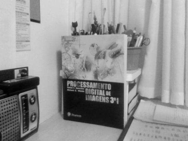
Depending on the choice of $h$, the result of the digital convolution can be one of many. We can mainly distinguish the effects of blurring and sharpening filters (yes, corresponding to low-pass or high-pass filters in the frequency domain).
Blurring filters cause the well-known “blur” effect in the image. They achieve this effect by using convolution sums to approximate the pixel intensity of the resulting image by averages of the pixels in their neighborhood, effectively smoothing abrupt transitions. The main examples are the box blur and the gaussian blur.
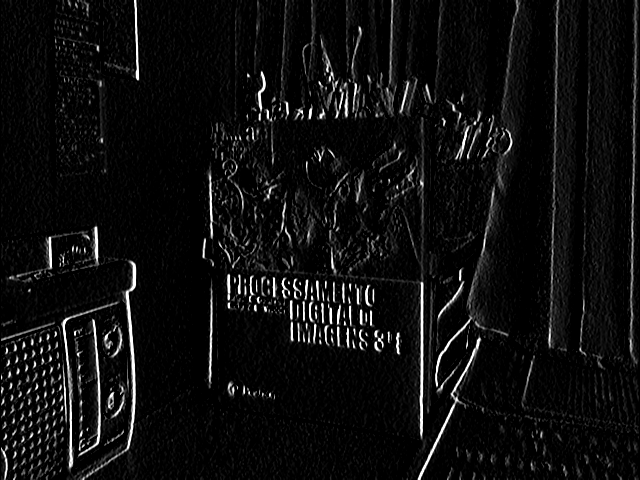
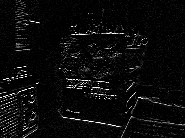
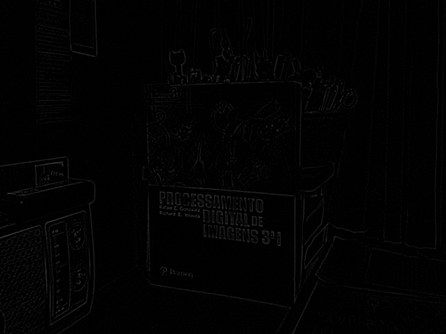
Sharpening filters produce the opposite effect: they use the convolution sum to calculate differences in the pixel neighborhood and enhance abrupt transitions, being widely used as edge detectors. Sobel filters are well-known examples of edge detection in specific directions (horizontal or vertical) and can even be used to estimate magnitude and direction of gradient vectors in images. Another classical example is the laplacian filter, which estimates the laplacian operator ($\nabla^2=\partial_x^2+\partial_y^2$) in the neighborhood of each pixel, detecting edges in all directions.
If we represent the kernels as square matrices 3x3, they are:
- Box Blur
\[
h_B = \frac{1}{9}
\begin{pmatrix}
1 & 1 & 1 \
1 & 1 & 1 \
1 & 1 & 1 \end{pmatrix} \] - Gaussian Blur
\[
h_G=\frac{1}{16}
\begin{pmatrix}
1 & 2 & 1 \
2 & 4 & 2 \
1 & 2 & 1 \end{pmatrix} \] - Sobel Filter
\[
h_x=
\begin{pmatrix}
-1 & 0 & 1 \
-2 & 0 & 2 \
-1 & 0 & 1 \end{pmatrix}, \qquad h_y= \begin{pmatrix} -1 & -2 & -1 \
0 & 0 & 0 \
1 & 2 & 1 \end{pmatrix} \] - Laplacian Filter
\[
h_\ell=
\begin{pmatrix}
0 & -1 & 0 \
-1 & 4 & -1 \
0 & -1 & 0 \end{pmatrix} \]
Filtering with OpenCV
In OpenCV, the function that will allow us to perform digital convolutions to filter images in the spatial domain is filter2D. But beware, what filter2D computes is the correlation between the two given matrices!
filtered = cv2.filter2D(image, depth, kernel)
Here, besides the image, the necessary arguments are depth, which specifies the type of the output (-1 for the same type as the input), and kernel, the 2D array representing the filter matrix $h^T(x,y)$. When the kernel is symmetrical, $h(x,y)=h^T(x,y)$ and we don’t have to worry too much about that.
Using multiple filters simultaneously
1
2
3
4
5
6
7
8
9
10
11
12
13
14
15
16
17
18
19
20
21
22
23
24
25
26
27
28
29
30
31
32
33
34
35
36
37
38
39
40
41
42
43
44
45
46
47
48
49
50
import cv2
import numpy as np

def menu():
    print("\npress a key to toggle a filter:"
          "\nb - box"
          "\ng - gaussian"
          "\nv - vertical"
          "\nh - horizontal"
          "\nl - laplacian"
          "\nx - reset all"
          "\nesc - exit")

cap = cv2.VideoCapture(0)
assert cap.isOpened(), 'UNAVAILABLE CAMERA'
# defining the kernels
box     = np.array([[1, 1, 1], [1, 1, 1], [1, 1, 1]]) / 9
gauss   = np.array([[1, 2, 1], [2, 4, 2], [1, 2, 1]]) / 16
horiz   = np.array([[-1, 0, 1], [-2, 0, 2], [-1, 0, 1]])
vert    = np.array([[-1, -2, -1], [0, 0, 0], [1, 2, 1]])
laplace = np.array([[0, -1, 0], [-1, 4, -1], [0, -1, 0]])

masks = dict(b=box, g=gauss, h=horiz, v=vert, l=laplace)
active = dict(b=False, g=False, h=False, v=False, l=False)

menu()
while True:
    _, image = cap.read()
    frame = cv2.cvtColor(image, cv2.COLOR_BGR2GRAY)
    cv2.imshow('original', frame)
    # apply all currently active filters in succession
    for key in masks.keys():
        if active[key]:
            frame = cv2.filter2D(frame, -1, masks[key])
    cv2.imshow('filtered', frame)
    # keyboard events
    key = cv2.waitKey(10)
    if key > 0:
        key = chr(key)
    # esc - exit
    if key == chr(27):
        break
    # x - reset all
    if key == 'x':
        menu()
        active = dict.fromkeys(active, False)
    # toggle filter
    if key in active.keys():
        menu()
        active[key] = not active[key]
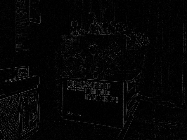
The results are as follows: