Image histograms and what they are for

In this tutorial we are going to try and understand what image histograms are and what they can be used for.

Histograms are our old acquaintances from statistics and basically consist of counting the frequency of occurrences of a certain event. In our case, we are interested in the brightness distribution of a digital image. A image histogram associates to each brightness value the number of pixels in the image with that given value.

The most immediate application of image histograms is the image thresholding operation: by analyzing the brightness distribution, the clusters of light/dark pixels are identified and a threshold is established from which the image can be binarized. But that’s not what this post is about; instead, we are going to investigate other histogram applications.

Equalization

The equalization operation consists in a special type of contrast adjustment. Its purpose is to turn the image’s brightness distribution in a (approximately) uniform distribution.

Statistically speaking, we can associate the histogram of image $f(x,y)$ to a probability mass function \[p_f(i) = p(f=i) = \frac{n_i}{n}\] where $n_i$ pixels out of $n$ have brightness equal to $i$. A cumulative distribution is thus defined as \[P_f(i) = \sum_{j=0}^{i}p_f(j)\] In order to make the image distribution uniform, its cumulative distribution should become linear; all we have to do is \[g(x,y) = P_f(f(x,y)) \times (L-1)\] and the equalized image $g(x,y)$ will have zero brightness (black) where $f(x,y)$ is minimum, and brightness $(L-1)$ (pure white) where $f(x,y)$ is maximum.

Capturing video from your computer camera

We’re now ready to implement our own image equalization algorithm in Python. But before that, let’s see how to capture video in real time using OpenCV with devices connected to your computer. This is done through the VideoCapture class, which creates a video capture object from a camera identification parameter. This class has an isOpened method that can be used to test if the connection to the camera was successfully opened. In addition, we’ll use the read method to capture a frame from the camera. All this is done within a loop until the ESC key is pressed:

import cv2

cap = cv2.VideoCapture(0)
assert cap.isOpened(), 'UNAVAILABLE CAMERA'
while True:
    ret, frame = cap.read()
    cv2.imshow('camera video', frame)
    if cv2.waitKey(20) & 0xFF == 27:
        cv2.destroyAllWindows()
        break

The code snippet above only captures and shows in real time the frames as they are captured. When we’re done using it, the VideoCapture object can be freed using the release function:

cap.release()

Calculating the histogram: NumPy vs OpenCV

The computation of the histogram from the counting of occurrences of image intensity levels is a simple operation that can be implemented in many trivial ways. However, these very naive implementations can lead to unnecessarily high execution times, which is not ideal (especially for real-time operations).

NumPy has a function called histogram which takes a one-dimensional array, the number of bins, and the lower and upper bin range as parameters. For a 256-level grayscale image, its histogram could be directly calculated as follows:

hist, bins = np.histogram(image.ravel(), bins=256, range=(0, 256))

where hist is the array with the counts we want and bins is simply an array of edges between each bin (0, 1, …, 256). For one-dimensional histogams (like the ones we are computing here) it is more efficient to use the bincount function with the parameter minlength set to 256:

hist = np.bincount(image.ravel(), minlength=256)

Compared to histogram, running bincount can be up to 10x faster. However, OpenCV itself has a histogram calculation function, about 40x more efficient than the NumPy version! This is generally true for most of the features implemented in OpenCV, which are not only optimized for image processing, but are also implemented in C/C++ behind the scenes. The OpenCV function that will be of interest to us is calcHist, taking the image, the channel in which you want to compute the histogram, a mask of a particular region of the image in which you want to compute the histogram, the number of bins (256), and the range (0 to 256):

hist = cv2.calcHist([image], [0], None, [256], [0, 256])

The above syntax should be used exactly this way, with each argument begin a bracket-delimited list, or OpenCV will raise a SystemError stating that the function returned NULL.

Using OpenCV to plot the histograms on the image itself

For a better visualization, we can plot the histograms together with each frame. To do this we can use the OpenCV line function to draw vertical lines and plot the entire histogram on a 256 pixel wide image:

def plot_hist(hist, color):
    norm_hist = hist * (height / np.max(hist))
    norm_hist = norm_hist.astype(int)
    img = np.zeros((height, 256, 3))
    for i in range(256):
        cv2.line(img, (i, height), (i, height - norm_hist[i]), color)
    return img

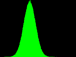
In the above code, the variable height defines the height in pixels (number of rows) of the image that will hold the histogram plot, and the variable norm_hist normalizes the histogram range between zero and height. After that, for each brightness value i between 0 and 255 a vertical line is drawn from the point (i, height) on the last row of the image to the corresponding point norm_hist[i] pixels above. By testing this function with the histogram of a random image with Gaussian distribution, we obtain:

height = 192
noise = np.random.normal(loc=100, scale=20, size=(640, 480)).astype(np.uint8)
hist = cv2.calcHist([noise], [0], None, [256], [0, 256])
hist_img = plot_hist(hist, (0, 255, 0))
cv2.imwrite('histogram.png', hist_img)

Simplifying the process: cv2.equalizeHist

Of course OpenCV already has an implementation of the complete equalization process through the equalizeHist function. This function basically takes as input the original image and returns the image already equalized:

equalized = cv2.equalizeHist(original)

However, it only works with grayscale images, since it operates with a single channel histogram. We can get around this by considering the three channels of a color image as being independent and equalizing each one individually.

_, original = cap.read()
r, g, b = cv2.split(original)
eqr = cv2.equalizeHist(r)
eqg = cv2.equalizeHist(g)
eqb = cv2.equalizeHist(b)
equalized = cv2.merge([eqr, eqg, eqb])

The split function basically transforms the color image represented by an array with shape (M, N, 3) into three separate arrays shaped (M, N), while merge does the reverse.

Putting it all together

Finally, we can use everything we have discussed so far and create a program that:

• capture real-time camera frames,
• equalize the original image,
• compute the histograms of both images, and
• plot the histograms on rectangular regions of the images themselves.

import cv2
import numpy as np

cap = cv2.VideoCapture(0)
assert cap.isOpened(), 'UNAVAILABLE CAMERA'

def get_hist(img):
    hist = cv2.calcHist([img], [0], None, [256], [0, 256])
    return hist.ravel()

height = 128
def plot_hist(hist, color):
    norm_hist = hist * (height / np.max(hist))
    norm_hist = norm_hist.astype(int)
    img = np.zeros((height, 256, 3))
    for i in range(256):
        cv2.line(img, (i, height), (i, height - norm_hist[i]), color)
    return img

while True:
    _, original = cap.read()
    r, g, b = cv2.split(original)
    eqr = cv2.equalizeHist(r)
    eqg = cv2.equalizeHist(g)
    eqb = cv2.equalizeHist(b)
    equalized = cv2.merge([eqr, eqg, eqb])
    histR = get_hist(r)
    histG = get_hist(g)
    histB = get_hist(b)
    original[        :  height, :256] = plot_hist(histR, (0, 0, 255))
    original[  height:2*height, :256] = plot_hist(histG, (0, 255, 0))
    original[2*height:3*height, :256] = plot_hist(histB, (255, 0, 0))
    eq_histR = get_hist(eqr)
    eq_histG = get_hist(eqg)
    eq_histB = get_hist(eqb)
    equalized[        :  height, :256] = plot_hist(eq_histR, (0, 0, 255))
    equalized[  height:2*height, :256] = plot_hist(eq_histG, (0, 255, 0))
    equalized[2*height:3*height, :256] = plot_hist(eq_histB, (255, 0, 0))
    cv2.imshow('original', original)
    cv2.imshow('equalized', equalized)
    if cv2.waitKey(20) & 0xFF == 27:
        break

The result should be something like

Result of running the equalization code above. Original image (left) and equalized (right).

Motion Detection

A less usual application of image histograms may be in motion detection. After all, while comparisons between consecutive images will always have tiny differences due to noise and small variations in camera position, the brightness distribution of the image is not as sensitive to these effects. Thus, comparing histograms of consecutive images can be an effective motion detection strategy.

Creating a comparison metric between consecutive histograms

In order to decide if there really was movement or not, it is necessary to establish a way to quantify the differencces between two consecutive histograms. One way could be, for example, to calculate the mean square error:

mse = np.mean(np.square(hist - previous))

From there, an error threshold could be calibrated, above which the movement would be detected.

Using cv2.compareHist and its metrics

OpenCV provides us with a function to compare two histograms called compareHist. In addition to the histograms in question, this function takes as an argument which metric of comparison should be applied. In other words, compareHist returns the result of applying a “distance function” $d$ over the two histograms $h_1$ and $h_2$. The main metric functions are:

• Correlation (HISTCMP_CORREL) \[d(h_1,h_2) = \frac{\sum_i (h_1(i)-\bar{h_1})(h_2(i)-\bar{h_2})}{\sqrt{\sum_i (h_1(i)-\bar{h_1})^2 \sum_i (h_2(i)-\bar{h_2})^2}}\]
• Chi-Squared (HISTCMP_CHISQR) \[d(h_1,h_2) = \sum_i\frac{(h_1(i) - h_2(i))^2}{h_1(i)}\]
• Intersection (HISTCMP_INTERSECT) \[d(h_1,h_2) = \sum_i\min(h_1(i), h_2(i))\]

There are also more sophisticated metrics, such as the Hellinger distance (related to the Bhattacharyya coefficient) or the Kullback-Leibler divergence, but for our purposes we can choose one of these three simpler options.

Changes in the correlation coefficient between consecutive frames are usually very small, making it difficult to estimate a threshold. Similarly, because histograms don’t change a lot between frames, their intersection always remains at high levels. Hence, for our application we will choose to use the chi-squared metric to compare consecutive histograms.

End result

To make our lives easier, let’s deal with the image on a grayscale. This way, we’ll have to worry about the variations over just one histogram. We are also going to use the functions we defined above to plot the normalized histogram in the upper left corner of the image, along with a “difference histogram”.

To record the calculated difference between the current and previous histograms, we’ll use the OpenCV putText function to write the value over the histogram. We are also going to use putText to write the message MOTION DETECTED whenever the distance is beyond the threshold that we can choose heuristically.

import cv2
import numpy as np

cap = cv2.VideoCapture(0)
assert cap.isOpened(), 'UNAVAILABLE CAMERA'

height = 128
def plot_hist(hist, color):
    hist = hist.astype(int)
    img = np.zeros((height, 256))
    for i in range(256):
        cv2.line(img, (i, height), (i, height - hist[i]), color)
    return img
    
threshold = 1000
previous = np.zeros((256, 1), np.float32)
while True:
    _, frame = cap.read()
    gray = cv2.cvtColor(frame, cv2.COLOR_BGR2GRAY)
    hist = cv2.calcHist([gray], [0], None, [256], [0, 256])
    diff = hist - previous
    norm_hist = hist * (height / np.max(hist))
    norm_diff = diff * (height / np.max(hist))
    gray[      :  height, :256] = plot_hist(norm_hist.ravel(), 127)
    gray[height:2*height, :256] = plot_hist(norm_diff.ravel(), 127)
    dist = cv2.compareHist(hist, previous, cv2.HISTCMP_CHISQR)
    previous = hist.copy()
    cv2.putText(gray, '%.2f' % dist, (0, 3*height//2), fontScale=2,
                fontFace=cv2.FONT_HERSHEY_SIMPLEX, thickness=2,
                color=255, lineType=cv2.LINE_AA)
    if dist > threshold:
        cv2.putText(gray, 'MOTION DETECTED', (50, 450), fontScale=2,
                    fontFace=cv2.FONT_HERSHEY_SIMPLEX, thickness=2,
                    color=255, lineType=cv2.LINE_AA)
    cv2.imshow('frame', gray)
    if cv2.waitKey(20) & 0xFF == 27:
        break

And here’s the detector at work: